Dataset Overview

Floating Car Data

This application analyzes truck travel time data on German freeway facilities using Floating Car Data (FCD) from 2019. In general, Floating Car Data (FCD) is generated by on-board units or navigation systems in vehicles and provides information on vehicle velocity over time (timestamp) and space (geocoordinates). Data providers typically offer either ‘raw’ FCD or aggregated FCD, such as percentiles of velocities over specific network elements. ‘Raw’ FCD, in this context, refers to data that can either track an individual vehicle's movement over time or be aggregated over specific network elements to provide an overview of traffic conditions. We utilize 'raw' FCD data for the year 2019, provided by ADAC . The ADAC collects FCD from various providers to monitor traffic conditions through their own systems. We do not have specific information on the providers from which the ADAC collects the data. Our sample comprises more than 25 billion data points. The number of FCD hits varies between months; approximately 2 billion FCD hits are recorded each month, with notably higher numbers in the summer months, which can be attributed to holiday traffic. The hourly distribution of FCD hits is relatively consistent across months and days, suggesting that the composition of the FCD sample is primarily influenced by fleets. Checking the daily distribution of the sample we can observe the formation of a plateau which is more common in truck traffic unlike to the observed daily patterns in passenger traffic, with two peaks during the morning and evening rush hours. In addition to the number of FCD hits and their hourly distribution, the examination of individual vehicles is of interest. For anonymization reasons, a vehicle can only be tracked in the FCD sample for 24 hours. Even in this context, the distribution of the number of vehicle IDs remains relatively constant, with approximately 15 million vehicle IDs. Given that we are using a raw FCD sample, it is essential to perform a network assignment and vehicle classification.

Network model

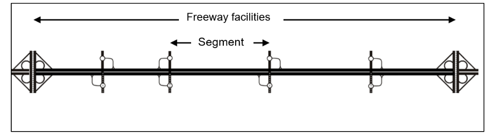
The network model, obtained from the Geofabrik for the year 2019, has been segmented to differentiate 3 aggregate levels. The smallest aggregate level is the 100 m-edge which is the basis for the network assignment algorithm; so the 100 m-edge serves as the aggregation level for the FCD to secure a certain. spatial resolution and plays also a crucial role for the interpolation algorithm conducted; The concept is taken from (Holthaus, o. J.). In general freeway facilities comprise basic, diverge, merge and weaving segments or intersections. (Forschungsgesellschaft für Straßen- und Verkehrswesen, 2015; Lemke, 2016) To enable the analysis of travel times at both segment and freeway facility levels, an algorithm was developed to segment the network model. This process required the classification of various motorway elements, including basic, diverging, merging, and weaving segments, as well as intersections. Based on this classification, 100- meter-edges were aggregated till they intersected with elements classified as basic, diverging, merging, or weaving segments. The freeway facilities were derived from the planning concept of the federal agency of Germany. (Bundesministerium für Verkehr und Digitales, 2018) The following figure depicts the distinction between freeway facilities and segments. (Geistefeldt, 2015)

Methodology

How to derive travel times?

• Network Assignment: Using OpenSourceRouting Machine (OSRM) with Hidden Markov Models for accurate map matching
• Vehicle Classification: K-means clustering to distinguish between truck and passenger vehicle patterns
• Adapative Smoothing Method: Given the spatial and temporal variability in FCD penetration, interpolation is necessary to derive a continuous velocity function for specific time intervals and spatial resolutions. The sample includes approximately 19 truck FCD hits per kilometre of freeway per hour, which is insufficient to detect traffic disruptions and their temporal and spatial fluctuations. Therefore, the Adaptive Smoothing Method (ASM) by (Treiber and Helbing, 2002; Treiber and Kesting, 2010) is applied. Spatiotemporal interpolation algorithms provide continuous average velocities as functions of space and time, derived from traffic stations. Since the FCD sample is assigned to the network model, they can be spatially and temporally aggregated, making the methodology applicable to the available data.(Treiber and Helbing, 2002; Treiber and Kesting, 2010)
• Dynamic travel times: As the path of a segment or freeway facility is predefined , we start at the first 100m-edge of a segment or freeway facility and end at the last 100m-edge, along with a particular start time—for example, 08:00 hours (this can be adjusted based on requirements). Starting from the initial time, as the segments and freeway facilities are divided into 100m-edges we calculate the travel time for each 100m-edge at the starting time, keeping track of the cumulative travel time spent as we move from one 100m-edge to the next. This process continues until the total time reaches 10 minutes (assuming the last 100m-edge has not yet been reached). At this point, we update the velocity to reflect the conditions at 08:10 hours and repeat the process for the next 10-minute interval. This cycle of updating the velocity every 10 minutes and calculating travel times for each segment continues until the last element is reached. The 10-minute interval can also be adjusted based on the desired level of detail.

Further explanations

Traffic times

• Morning Rush: Between 06:00 and 09:00
• Morning Off-Peak: Between 04:00 and 06:00
• Normal traffic time: Between 09:00 and 16:00
• Evening Rush: Between 16:00 and 19:00
• Evening Off-Peak: 19:00 and 21:00

Key Performance Indicators

Academic Reference

The methodologies and findings presented in this application are detailed in the following publication: